You can group and subtotal columns of merged data using the “Group” and “Subtotal” parameters. For more information, see Excel Merge Field Parameters.
In the following example, we demonstrate how to group and subtotal Opportunity Line Items by Product Family.
For Excel to sort the fields properly post merge, sort by the same field on your query or report.
Step 1: Non-Grouped Template
Start with a simple template that displays the non-grouped data.
Template:
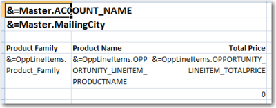
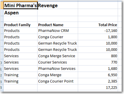
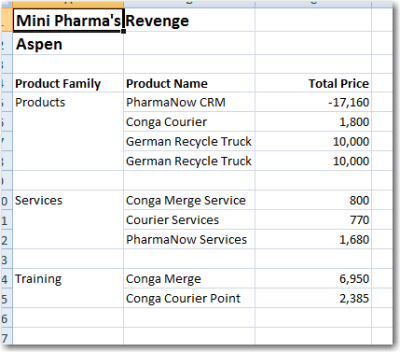
Output:
Step 2: Group by Product Family
Next, modify the merge field that represents the Product Family. Add the parameter to group on that field and to skip a row between Product Family values to make room for a subtotal (in a subsequent step).
Sort your report by the same field you are using as a group. For example, sort the example report by Product Family.
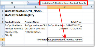
Template:
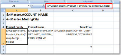
Output:
Using the SUBTOTAL9 function as depicted below ensures that each group maintains a subtotal and prevents blank lines from appearing below the merge results.
Step 3: Subtotal on Price
Next, insert a formula to subtotal on Total Price. We added bold formatting to the formula to emphasize it.
The Subtotal function must evaluate the same field on which you are grouping. For example, if the field being grouped on is Product Family, then the group parameter will state &=OppLineItems.Product_Family(Group:Merge, Skip:1), and Subtotal will be entered as &=Subtotal9:OppLineItems.Product_Family.
Template:
Output:
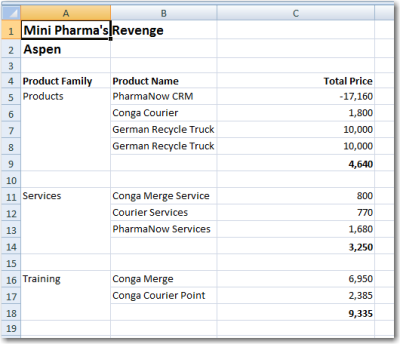
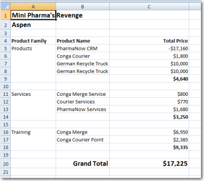
Notice each subtotal in bold text.
Step 4: Compute Grand Total
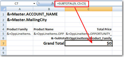
Finally, insert a formula to find the grand total of the Price column. Do not use the =SUM function to add this column, as it will include the subtotal values in the result. Instead, we’ll include the Excel formula:
=SUBTOTAL(9, C5:C5)
We also added a label for the total (“Grand Total”) and formatted the values as currency (USD).
Template:
Output: